Plot method for the simulations of a fgpm model

This method displays the simulated output values delivered by a funGp Gaussian process model.

# S3 method for simulate.fgpm
plot(x, y = NULL, detail = NA, ...)

Arguments

x

An object with S3 class simulate.fgpm as created by simulate,fgpm-method.

y

Not used.

detail

An optional character string specifying the data elements that should be included in the plot, to be chosen between "light" and "full". A light plot will include only the simulated values, while a full plot will also include the predicted mean and confidence bands at the simulation points. This argument will only be used if full simulations (including the mean and confidence bands) are provided, otherwise it will be ignored. See simulate,fgpm-method for more details on the generation of light and full simulations.

...

Additional arguments affecting the display. The following typical graphics parameters are valid entries: xlim, ylim, xlab, ylab, main. The boolean argument legends can also be included in any of the two lists in order to control the display of legends in the corresponding plot.

See also

* fgpm for the construction of funGp models;

* plot,fgpm-method for model diagnostic plots;

* predict,fgpm-method for predictions based on a funGp model;

* plot.predict.fgpm for prediction plots.

Author

José Betancourt, François Bachoc and Thierry Klein

Examples

# plotting light simulations________________________________________________
# building the model
set.seed(100)
n.tr <- 25
sIn <- expand.grid(x1 = seq(0, 1, length = sqrt(n.tr)),
                   x2 = seq(0, 1, length = sqrt(n.tr)))
fIn <- list(f1 = matrix(runif(n.tr * 10), ncol = 10),
            f2 = matrix(runif(n.tr * 22), ncol = 22))
sOut <- fgp_BB3(sIn, fIn, n.tr)
m1 <- fgpm(sIn = sIn, fIn = fIn, sOut = sOut)
#> ** Presampling...
#> ** Optimising hyperparameters...
#> final  value 2.841058 
#> converged
#> The function value is the negated log-likelihood
#> ** Hyperparameters done!

# making light simulations
n.sm <- 100
sIn.sm <- as.matrix(expand.grid(x1 = seq(0, 1, length = sqrt(n.sm)),
                                x2 = seq(0, 1, length = sqrt(n.sm))))
fIn.sm <- list(f1 = matrix(runif(n.sm * 10), ncol = 10),
               f2 = matrix(runif(n.sm * 22), ncol = 22))
simsl <- simulate(m1, nsim = 10, sIn.sm = sIn.sm, fIn.sm = fIn.sm)

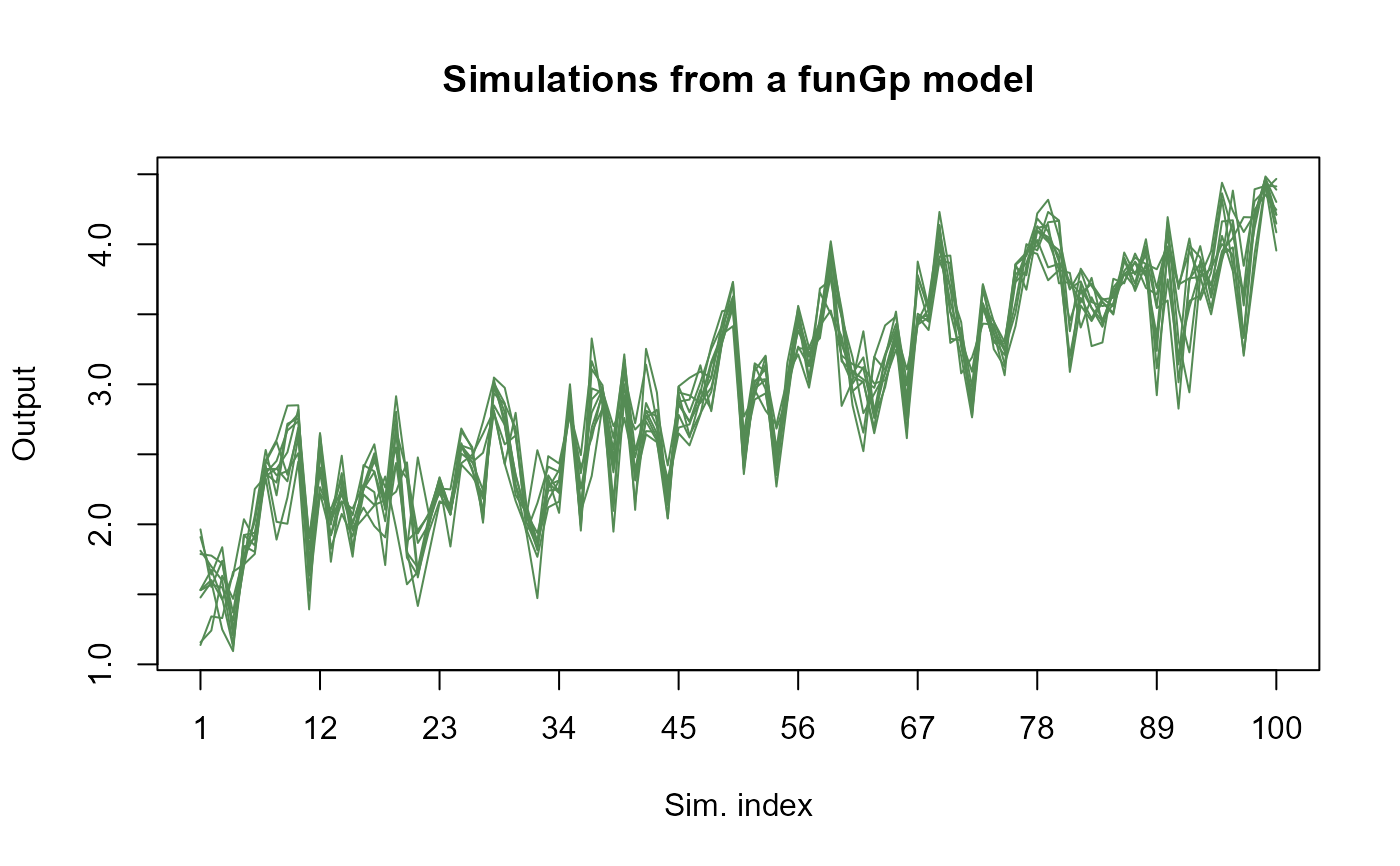
# plotting light simulations
plot(simsl)



# plotting full simulations_________________________________________________
# building the model
set.seed(100)
n.tr <- 25
sIn <- expand.grid(x1 = seq(0, 1, length = sqrt(n.tr)),
                   x2 = seq(0, 1, length = sqrt(n.tr)))
fIn <- list(f1 = matrix(runif(n.tr * 10), ncol = 10),
            f2 = matrix(runif(n.tr * 22), ncol = 22))
sOut <- fgp_BB3(sIn, fIn, n.tr)
m1 <- fgpm(sIn = sIn, fIn = fIn, sOut = sOut)
#> ** Presampling...
#> ** Optimising hyperparameters...
#> final  value 2.841058 
#> converged
#> The function value is the negated log-likelihood
#> ** Hyperparameters done!

# making full simulations
n.sm <- 100
sIn.sm <- as.matrix(expand.grid(x1 = seq(0, 1, length = sqrt(n.sm)),
                                x2 = seq(0, 1 ,length = sqrt(n.sm))))
fIn.sm <- list(f1 = matrix(runif(n.sm * 10), ncol = 10),
               f2 = matrix(runif(n.sm * 22), ncol = 22))
simsf <- simulate(m1, nsim = 10, sIn.sm = sIn.sm, fIn.sm = fIn.sm,
                  detail = "full")

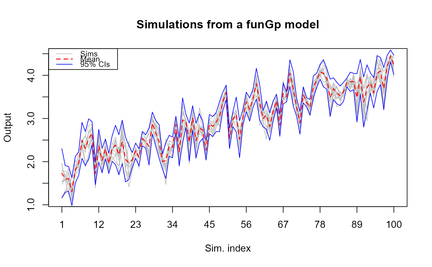
# plotting full simulations in "full" mode
plot(simsf)


# plotting full simulations in "light" mode
plot(simsf, detail = "light")