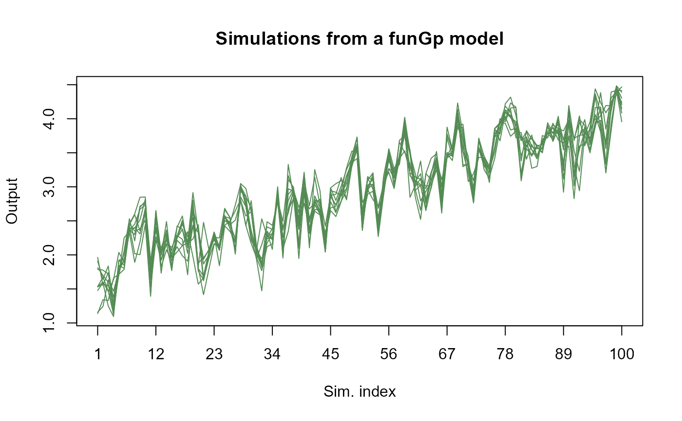
Random sampling from a fgpm model — simulate,fgpm-method • funGp

This method enables simulation of Gaussian process values at any given set of points based on a pre-built fgpm model. Check fgpm for information on how to create funGp models.

# S4 method for fgpm
simulate(
  object,
  nsim = 1,
  seed = NULL,
  sIn.sm = NULL,
  fIn.sm = NULL,
  nugget.sm = 0,
  detail = c("light", "full"),
  ...
)

Arguments

object: An object of class fgpm corresponding to the funGp model from which simulations must be performed.
nsim: An optional integer indicating the number of samples to produce. Default is 1.
seed: An optional value interpreted as an integer, that will be used as argument of set.seed just before simulating the response values.
sIn.sm: An optional matrix of scalar input coordinates at which the output values should be simulated. Each column is interpreted as a scalar input variable and each row as a coordinate. Either scalar input coordinates (sIn.sm), functional input coordinates (fIn.sm), or both must be provided.
fIn.sm: An optional list of functional input coordinates at which the output values should be simulated. Each element of the list is interpreted as a functional input variable. Every functional input variable should be provided as a matrix with one curve per row. Either scalar input coordinates (sIn.sm), functional input coordinates (fIn.sm), or both must be provided.
nugget.sm: An optional number corresponding to a numerical nugget effect. If provided, this number is added to the main diagonal of the simulation covariance matrix in order to prevent numerical instabilities during Cholesky decomposition. A small number in the order of 1e-8 is often enough. Default is 0.
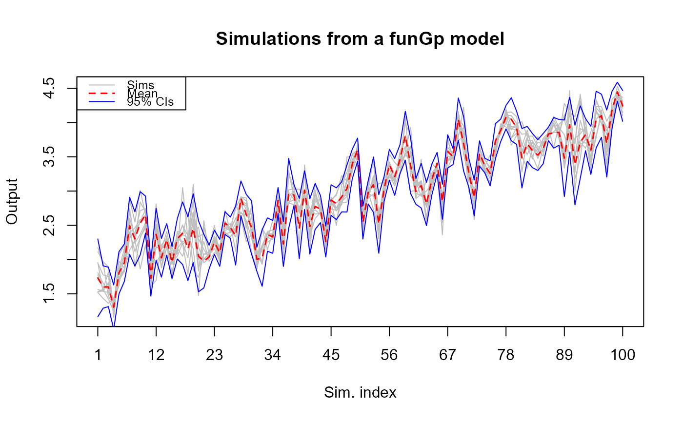
detail: An optional character specifying the extent of information that should be delivered by the method, to be chosen between "light" (default) and "full". Light simulations produce a matrix of simulated output values, with as many rows as requested random samples. Full simulations produce a list with the matrix of simulated output values, along with the predicted mean, standard deviation and limits of the 95% confidence intervals at the simulation points.
...: Not used.

Value

An object containing the data structures linked to simulations. For light simulations, the output will be a matrix of simulated output values, with as many rows as requested random samples. For full simulations, the output will be a list with the matrix of simulated output values, along with the predicted mean, standard deviation and limits of the 95% confidence intervals at the simulation points.

Author

José Betancourt, François Bachoc, Thierry Klein and Jérémy Rohmer

Examples

# light simulations _______________________________________________________________________
# building the model
set.seed(100)
n.tr <- 25
sIn <- expand.grid(x1 = seq(0,1,length = sqrt(n.tr)), x2 = seq(0,1,length = sqrt(n.tr)))
fIn <- list(f1 = matrix(runif(n.tr*10), ncol = 10), f2 = matrix(runif(n.tr*22), ncol = 22))
sOut <- fgp_BB3(sIn, fIn, n.tr)
m1 <- fgpm(sIn = sIn, fIn = fIn, sOut = sOut)
#> ** Presampling...
#> ** Optimising hyperparameters...
#> final  value 2.841058 
#> converged
#> The function value is the negated log-likelihood
#> ** Hyperparameters done!

# generating input data for simulation
n.sm <- 100
sIn.sm <- as.matrix(expand.grid(x1 = seq(0,1,length = sqrt(n.sm)),
                                x2 = seq(0,1,length = sqrt(n.sm))))
fIn.sm <- list(f1 = matrix(runif(n.sm*10), ncol = 10), matrix(runif(n.sm*22), ncol = 22))

# making light simulations
m1.sims_l <- simulate(m1, nsim = 10, sIn.sm = sIn.sm, fIn.sm = fIn.sm)

# plotting light simulations
plot(m1.sims_l)



# full simulations ________________________________________________________________________
# building the model
set.seed(100)
n.tr <- 25
sIn <- expand.grid(x1 = seq(0,1,length = sqrt(n.tr)), x2 = seq(0,1,length = sqrt(n.tr)))
fIn <- list(f1 = matrix(runif(n.tr*10), ncol = 10), f2 = matrix(runif(n.tr*22), ncol = 22))
sOut <- fgp_BB3(sIn, fIn, n.tr)
m1 <- fgpm(sIn = sIn, fIn = fIn, sOut = sOut)
#> ** Presampling...
#> ** Optimising hyperparameters...
#> final  value 2.841058 
#> converged
#> The function value is the negated log-likelihood
#> ** Hyperparameters done!

# making full simulations
m1.sims_f <- simulate(m1, nsim = 10, sIn.sm = sIn.sm, fIn.sm = fIn.sm, detail = "full")

# checking content of the list
summary(m1.sims_f)
#>         Length Class  Mode   
#> sims    1000   -none- numeric
#> mean     100   -none- numeric
#> sd       100   -none- numeric
#> lower95  100   -none- numeric
#> upper95  100   -none- numeric

# ~R output:~
#         Length Class  Mode
# sims    1000   -none- numeric
# mean     100   -none- numeric
# sd       100   -none- numeric
# lower95  100   -none- numeric
# upper95  100   -none- numeric

# plotting full simulations in full mode
plot(m1.sims_f)


# plotting full simulations in light mode
plot(m1.sims_f, detail = "light")

Random sampling from a `fgpm` model

Arguments

Value

See also

Author

Examples